Learning how to compute time derivatives

Differentiation methods

This notebook explores various choices of differentiation methods that can be used with PyKoopman’s KoopmanContinuous class.

The optional parameter differentiator of the KoopmanContinuous class allows one to pass in custom time differentiation methods. differentiator should be callable with the call signature differentiator(x, t) where x is a 2D numpy ndarray with each example occupying a row and t is a 1D numpy ndarray containing the points in time for each row in x.

Two common options for differentiator are 1) Methods from the derivative package, called via the pykoopman.differentiation.Derivative wrapper. 2) Entirely custom methods.

import sys
sys.path.append('../src')

from platform import python_version
python_version()

'3.10.11'

from derivative import dxdt
import matplotlib.pyplot as plt
import numpy as np

import pykoopman as pk
from pydmd import DMD

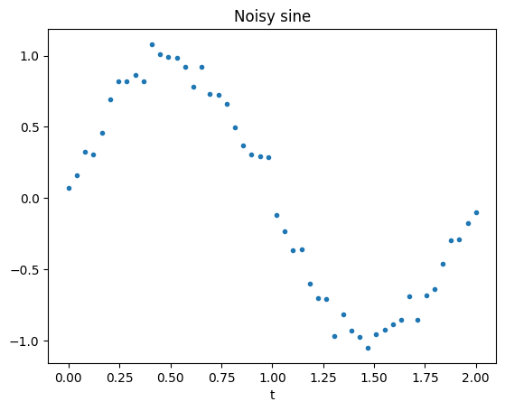
t = np.linspace(0, 2, 50)
x = np.sin(np.pi * t) + 0.1 * np.random.standard_normal(t.shape)
x_dot = np.pi * np.cos(np.pi *  t)

plt.plot(t, x, '.')
plt.xlabel('t')
plt.title('Noisy sine');

Derivative package

All of the robust differentiation methods in the derivative package are available with the pykoopman.differentiation.Derivative wrapper class. One need only pass in the same keyword arguments to Derivative that one would pass to derivative.dxdt.

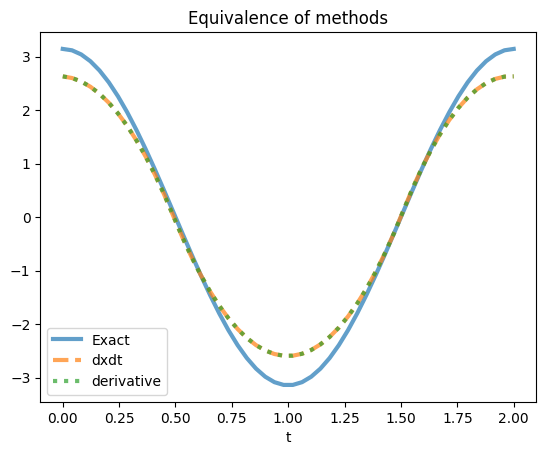
For example, we’ll compute the derivative of a noisy sine function with dxdt and Derivative using spline-based numerical differentiation and compare the results.

kws = dict(kind='spline', s=0.7, periodic=True)
x_dot_dxdt = dxdt(x, t, **kws)
x_dot_derivative = pk.differentiation.Derivative(**kws)(x, t)

plot_kws = dict(alpha=0.7, linewidth=3)
plt.plot(t, x_dot, label='Exact', **plot_kws)
plt.plot(t, x_dot_dxdt, '--', label='dxdt', **plot_kws)
plt.plot(t, x_dot_derivative, ':', label='derivative', **plot_kws)
plt.xlabel('t')
plt.title('Equivalence of methods')
plt.legend();

Custom differentiation method

We also have the option of defining a fully custom differentiation function. Here we’ll wrap numpy’s gradient method. We can pass this method into the differentiator argument of a KoopmanContinuous object.

from numpy import gradient

def diff(x, t):
    return gradient(x, axis=0)

dmd = DMD(svd_rank=2)
model = pk.KoopmanContinuous(differentiator=diff, regressor=dmd)
model.fit(x, dt=t[1]-t[0])

KoopmanContinuous(differentiator=<function diff at 0x000001F2B61B2D40>,
                  observables=Identity(),
                  regressor=PyDMDRegressor(regressor=<pydmd.dmd.DMD object at 0x000001F29514A410>))

In a Jupyter environment, please rerun this cell to show the HTML representation or trust the notebook.
On GitHub, the HTML representation is unable to render, please try loading this page with nbviewer.org.