Successful examples of using Dynamic mode decomposition on PDE system

We apply dynamic mode decomposition (DMD) to several PDE systems from J. Nathan Kutz, J. L. Proctor, and S. L. Brunton, “Applied Koopman Theory for Partial Differential Equations and Data-Driven Modeling of Spatio-Temporal Systems,” Complexity, vol. 2018, no. ii, pp. 1–16, 2018.): 1) 1D viscous Burgers equation. 2) 1D nonlinear schrodinger equation

In these two examples, DMD works because the inherent dynamics is both low rank and linear.

We first import the pyKoopman package and other packages for plotting and matrix manipulation.

import sys
sys.path.append('../src')

%matplotlib inline
import matplotlib.pyplot as plt
import numpy as np
import warnings
warnings.filterwarnings('ignore')

import matplotlib.cm as cm
from mpl_toolkits.mplot3d import Axes3D

import pykoopman as pk

1. Viscous Burgers equation

\[u_t + u u_x = \nu u_{xx}\]

where periodic boundary condition is used on \([-15,15]\). Initial condition follows \(u(x,0)=e^{-(x+2)^2}\).

• use vbe.simulate to run simulation in order to get the training data

• use vbe.visualize_data to see how data evolves in space and time

• use vbe.visualize_state_space to see the data distribution in the first 3 PCA directions

from pykoopman.common import vbe

n = 256
x = np.linspace(-15, 15, n, endpoint=False)
u0 = np.exp(-(x+2)**2)
# u0 = 2.0 / np.cosh(x)
# u0 = u0.reshape(-1,1)
n_int = 3000
n_snapshot = 30
dt = 30. / n_int
n_sample = n_int // n_snapshot

model_vbe = vbe(n, x, dt=dt, L=30)
X, t = model_vbe.simulate(u0, n_int, n_sample)
delta_t = t[1]-t[0]

model_vbe.visualize_data(x, t, X)
model_vbe.visualize_state_space(X)

print("data shape = ",X.shape)

data shape =  (30, 256)

Run a vanilla DMD with just rank = 5. First, we import DMD regressor, feed it into Koopman. Second, we use model.fit to fit the data

from pydmd import DMD

dmd = DMD(svd_rank=5)
model = pk.Koopman(regressor=dmd)
model.fit(X, dt=delta_t)

Koopman(observables=Identity(),
        regressor=PyDMDRegressor(regressor=<pydmd.dmd.DMD object at 0x00000216CD9AF8B0>))

In a Jupyter environment, please rerun this cell to show the HTML representation or trust the notebook.
On GitHub, the HTML representation is unable to render, please try loading this page with nbviewer.org.

Check spectrum

Just use model.koopman_matrix to get the Koopman matrix

K = model.A

# Let's have a look at the eigenvalues of the Koopman matrix
evals, evecs = np.linalg.eig(K)
evals_cont = np.log(evals)/delta_t

fig = plt.figure(figsize=(4,4))
ax = fig.add_subplot(111)
ax.plot(evals_cont.real, evals_cont.imag, 'bo', label='estimated',markersize=5)


# ax.set_xlim([-0.1,1])
# ax.set_ylim([2,3])
plt.legend()
plt.xlabel(r'$Re(\lambda)$')
plt.ylabel(r'$Im(\lambda)$')
# print(omega1,omega2)

Text(0, 0.5, '$Im(\\lambda)$')

Define plotting function

def plot_pde_dynamics(x, t, X, X_pred, title_list, ymin=0, ymax=1):

    fig = plt.figure(figsize=(12, 8))

    ax = fig.add_subplot(131, projection='3d')
    for i in range(X.shape[0]):
        if X.dtype != 'complex':
            ax.plot(x, X[i], zs=t[i], zdir='t')
        else:
            ax.plot(x, abs(X[i]), zs=t[i], zdir='t')
    ax.set_ylim([ymin, ymax])
    ax.view_init(elev=35., azim=-65, vertical_axis='y')
    if X.dtype != 'complex':
        ax.set(ylabel=r'$u(x,t)$', xlabel=r'$x$', zlabel=r'time $t$')
    else:
        ax.set(ylabel=r'mag. of $u(x,t)$', xlabel=r'$x$', zlabel=r'time $t$')

    plt.title(title_list[0])

    ax = fig.add_subplot(132, projection='3d')
    for i in range(X.shape[0]):
        if X.dtype != 'complex':
            ax.plot(x, X_pred[i], zs=t[i], zdir='t')
        else:
            ax.plot(x, abs(X_pred[i]), zs=t[i], zdir='t')
    ax.set_ylim([ymin, ymax])
    ax.view_init(elev=35., azim=-65, vertical_axis='y')
    if X.dtype != 'complex':
        ax.set(ylabel=r'$u(x,t)$', xlabel=r'$x$', zlabel=r'time $t$')
    else:
        ax.set(ylabel=r'mag. of $u(x,t)$', xlabel=r'$x$', zlabel=r'time $t$')
    plt.title(title_list[1])

    ax = fig.add_subplot(133, projection='3d')
    for i in range(X.shape[0]):
        if X.dtype != 'complex':
            ax.plot(x, X_pred[i]-X[i], zs=t[i], zdir='t')
        else:
            ax.plot(x, abs(X_pred[i]-X[i]), zs=t[i], zdir='t')
    ax.set_ylim([ymin, ymax])
    ax.view_init(elev=35., azim=-65, vertical_axis='y')
    if X.dtype != 'complex':
        ax.set(ylabel=r'$u(x,t)$', xlabel=r'$x$', zlabel=r'time $t$')
    else:
        ax.set(ylabel=r'mag. of $u(x,t)$', xlabel=r'$x$', zlabel=r'time $t$')
    plt.title(title_list[2])

run inference using model.simulate

X_predicted = np.vstack((X[0], model.simulate(X[0], n_steps=X.shape[0] - 1)))
plot_pde_dynamics(x,t,X, X_predicted, ['Truth','DMD-rank:'+str(model.A.shape[0]),'Residual'])

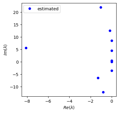
2. nonlinear schrodinger equation

\[iu_t + 0.5u_{xx} + u|u|^2 = 0\]

periodic boundary condition in \([-15,15]\) with initial condition as \(2.0 / \cosh(x)\)

from pykoopman.common import nlse

n = 512
x = np.linspace(-15, 15, n, endpoint=False)
u0 = 2.0 / np.cosh(x)
# u0 = u0.reshape(-1,1)
n_int = 10000
n_snapshot = 80  # in the original paper, it is 20, but I think too small
dt = np.pi / n_int
n_sample = n_int // n_snapshot

model_nlse = nlse(n, dt=dt, L=30)
X, t = model_nlse.simulate(u0, n_int, n_sample)

delta_t = t[1] - t[0]

model_nlse.visualize_data(x,t,X)
model_nlse.visualize_state_space(X)

Run a vanilla DMD with rank = 10

from pydmd import DMD

dmd = DMD(svd_rank=10)
model = pk.Koopman(regressor=dmd)
model.fit(X, dt=delta_t)

Koopman(observables=Identity(),
        regressor=PyDMDRegressor(regressor=<pydmd.dmd.DMD object at 0x00000216CFF6A4D0>))

In a Jupyter environment, please rerun this cell to show the HTML representation or trust the notebook.
On GitHub, the HTML representation is unable to render, please try loading this page with nbviewer.org.

K = model.A

# Let's have a look at the eigenvalues of the Koopman matrix
evals, evecs = np.linalg.eig(K)
evals_cont = np.log(evals)/delta_t

fig = plt.figure(figsize=(4,4))
ax = fig.add_subplot(111)
ax.plot(evals_cont.real, evals_cont.imag, 'bo', label='estimated',markersize=5)


# ax.set_xlim([-0.1,1])
# ax.set_ylim([2,3])
plt.legend()
plt.xlabel(r'$Re(\lambda)$')
plt.ylabel(r'$Im(\lambda)$')
# print(omega1,omega2)

Text(0, 0.5, '$Im(\\lambda)$')

X_predicted = np.vstack((X[0], model.simulate(X[0], n_steps=X.shape[0] - 1)))
plot_pde_dynamics(x,t,X, X_predicted,
                  ['Truth','DMD-rank:'+str(model.A.shape[0]),'Residual'],
                 0,4)

Conclusion: - DMD works very well for both systems - a simple linear fit can leads to visually very good reconstruction performance for nonlinear system

3. Revisiting cubic-quintic Ginzburg-Landau equation

Previously, we talked about a “Unsuccessful examples of using Dynamic mode decomposition on PDE system” and used an example of Ginzburg-Landau equation. In fact, we can make DMD work by simply truncating the initial transient phase.

from pykoopman.common import cqgle

n = 512
x = np.linspace(-10, 10, n, endpoint=False)
u0 = np.exp(-((x) ** 2))
# u0 = 2.0 / np.cosh(x)
# u0 = u0.reshape(-1,1)
n_int = 9000
n_snapshot = 300
dt = 40.0 / n_int
n_sample = n_int // n_snapshot

model_cqgle = cqgle(n, x, dt, L=20)
X, t = model_cqgle.simulate(u0, n_int, n_sample)

Here we truncate it after 100 time units

X = X[100:]

delta_t = t[1] - t[0]

# usage: visualize the data in physical space
model_cqgle.visualize_data(x, t, X)
model_cqgle.visualize_state_space(X)

In fact, there isn’t any change to the singular spectrum. But now you will see DMD will work amazingly on this problem

from pydmd import DMD

dmd = DMD(svd_rank=50)
model = pk.Koopman(regressor=dmd)
model.fit(X, dt=delta_t)

K = model.A

# Let's have a look at the eigenvalues of the Koopman matrix
evals, evecs = np.linalg.eig(K)
evals_cont = np.log(evals)/delta_t

fig = plt.figure(figsize=(4,4))
ax = fig.add_subplot(111)
# ax.plot(evals.real, evals.imag, 'bo', label='estimated', markersize=5)
ax.plot(evals_cont.real, evals_cont.imag, 'bo', label='estimated', markersize=5)
plt.legend()
plt.grid('on')
plt.xlabel(r'$Re(\lambda)$')
plt.ylabel(r'$Im(\lambda)$')

X_predicted = np.vstack((X[0], model.simulate(X[0], n_steps=X.shape[0]-1)))
plot_pde_dynamics(x, t, X, X_predicted,
                  ['Truth','DMD-rank:'+str(model.A.shape[0]),'Residual'], 0, 4)

Conclusion: - by removing some initial phase, we find vanilla DMD algorithm improves significantly. However, this means if one can stabilize DMD for general case, the algorith of Koopman can be much more powerful. This is the motivation for one of the authors to pursue learning stabilized Koopman opeartor.