Hankel Alternative View of Koopman Operator for Lorenz System

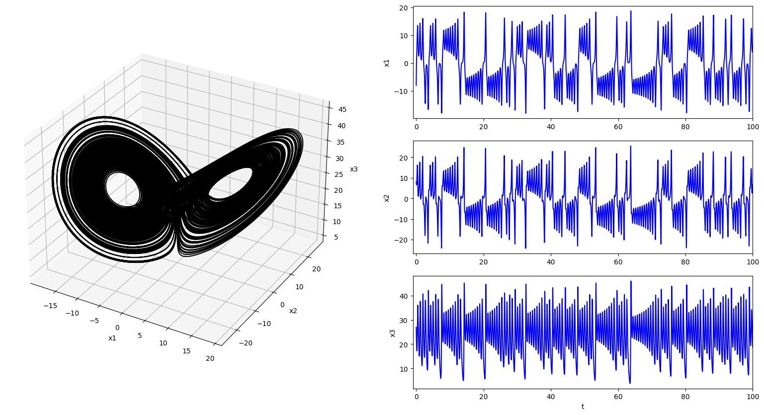
HAVOK combines delay embedding and Koopman theory to decompose chaotic dynamics into a linear model in the leading delay coordinates with forcing by low-energy delay coordinates; this is called the Hankel alternative view of Koopman (HAVOK) analysis. The method is illustrated on the chaotic Lorenz system (see Brunton, Brunton, Proctor, Kaiser & Kutz, “Chaos as an intermittently forced linear system”, Nature Communications 8(19), 2017):

\[\begin{split}\dot{x}_{1} = \sigma (x_2-x_1),\\ \dot{x}_2 = x_1(\rho-x_3)-x_2,\\ \dot{x}_3 = x_1x_2-\beta x_3\end{split}\]

with parameters \(\sigma=10\), \(\rho=28\), and \(\beta=8/3\).

import sys
sys.path.append('../src')

import numpy as np
from scipy import integrate
import matplotlib.pyplot as plt
from matplotlib.gridspec import GridSpec

import pykoopman as pk
from pykoopman.common import lorenz

Collect training data:

n_states = 3
x0 = [-8, 8, 27]  # initial condition
dt = 0.001  # timestep
t = np.linspace(dt, 200, 200000)  # time vector
x = integrate.odeint(lorenz, x0, t, atol=1e-12, rtol=1e-12)  # integrate ode

fig = plt.figure(figsize=(30,10))
gs = GridSpec(3, 3, figure=fig)
ax1 = fig.add_subplot(gs[:, 0], projection='3d')
ax1.plot3D(x[:, 0], x[:, 1], x[:, 2], '-k')
ax1.set_xlabel('x1')
ax1.set_ylabel('x2')
ax1.set_zlabel('x3')
ax1.grid()
ax2a = fig.add_subplot(gs[0, 1])
ax2a.plot(t, x[:, 0], '-b', label='x')
ax2a.set_ylabel('x1')
ax2a.set_xlim([-1, 100])
ax2b = fig.add_subplot(gs[1, 1])
ax2b.plot(t, x[:, 1], '-b', label='y')
ax2b.set_ylabel('x2')
ax2b.set_xlim([-1, 100])
ax2c = fig.add_subplot(gs[2, 1])
ax2c.plot(t, x[:, 2], '-b', label='z')
ax2c.set_ylabel('x3')
ax2c.set_xlabel('t')
ax2c.set_xlim([-1, 100])

(-1.0, 100.0)

HAVOK regression

The chaotic system is now modeled as a linear model in the leading delay coordinates, \({\bf v}:=[v_1, v_2, \ldots, v_{r-1}]^T\), with forcing by the low-energy, \(r\)th delay coordinate:

\[\dot{\bf v}(t) = {\bf A}{\bf v}(t) + {\bf B} v_r(t)\]

.

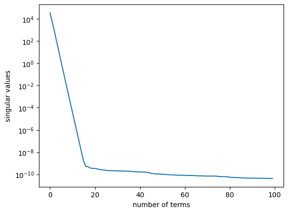
The observables chosen for the HAVOK model are time-delay coordinates of the first state coordinate \(x(t)\). The resulting data matrix is referred to as Hankel matrix. The number of delays is chosen to be \(100\). The HAVOK model computes a SVD of the Hankel matrix:

\[{\bf H} = {\bf U}{\bf \Sigma}{\bf V}^{*}.\]

In order to regress on the V’s delay coordinates, the corresponding time derivative (i.e. \(\dot{\bf v}\)) must be first estimated, e.g. using the 4th order central difference scheme. pyKoopman integrates the package derivative for differentiation, which provides a large suite of differentiation options for both clean and noisy data.

n_delays = 100-1

# # time delay on first and second component
# INDEX = [0,1]
# SVD_RANK = 15

# time delay only on first component
INDEX = [0]
SVD_RANK = 15

# # time delay only on second component
# INDEX = [1]
# SVD_RANK = 15

# # time delay on the third component
# INDEX = [2]
# SVD_RANK = 15

TDC = pk.observables.TimeDelay(delay=1, n_delays=n_delays)
HAVOK = pk.regression.HAVOK(svd_rank=SVD_RANK, plot_sv=True)
Diff = pk.differentiation.Derivative(kind='finite_difference', k=2)  # 4th order
# central difference

model = pk.KoopmanContinuous(observables=TDC, differentiator=Diff, regressor=HAVOK)
model.fit(x[:, INDEX], dt=dt)  # Compute model fit using training data

KoopmanContinuous(differentiator=Derivative(k=2, kind='finite_difference'),
                  observables=TimeDelay(n_delays=99),
                  regressor=HAVOK(plot_sv=True, svd_rank=15))

In a Jupyter environment, please rerun this cell to show the HTML representation or trust the notebook.
On GitHub, the HTML representation is unable to render, please try loading this page with nbviewer.org.

model.B.min()

-1.1467136340992274

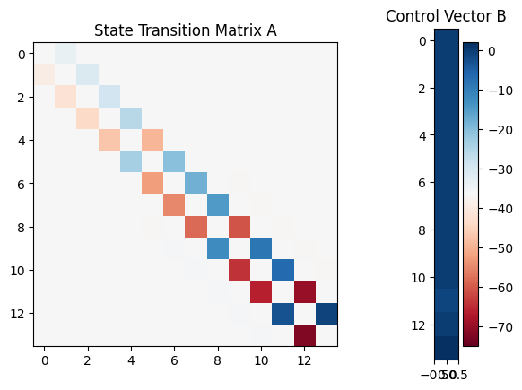
fig = plt.figure()
gs = GridSpec(1, 2, width_ratios=[3, 1])

ax0 = plt.subplot(gs[0])
im = ax0.imshow(model.A, aspect='equal', cmap=plt.get_cmap('RdBu'),vmin=-70, vmax=70)
ax0.set(title='State Transition Matrix A')

ax1 = plt.subplot(gs[1])
im = ax1.imshow(model.B, aspect='equal', cmap=plt.get_cmap('RdBu'), vmin=-75, vmax=2)
ax1.set(title='Control Vector B')
fig.colorbar(im, ax=ax1)

<matplotlib.colorbar.Colorbar at 0x131000e5ff0>

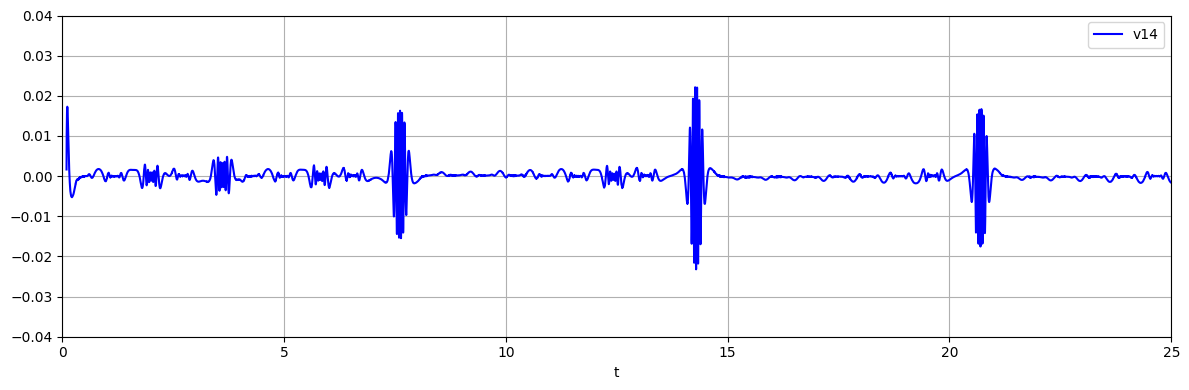
Extract forcing signal

which corresponds to the rth delay vector, here \(v_{14}\). The bursts correspond to lobe switching events of the chaotic Lorenz system.

u = model.regressor.forcing_signal

fig, axs = plt.subplots(1, 1, tight_layout=True, figsize=(12, 4))
axs.plot(t[n_delays:], u, '-b', label='v14')
axs.grid()
axs.set_xlabel('t')
axs.legend(loc='best')
plt.xlim([0, 25])
plt.ylim([-.04, .04])

(-0.04, 0.04)

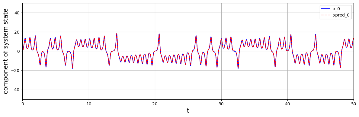
Prediction using the HAVOK model

Using the identified model with the forcing signal \(u=v_{14}\), it is possible to reconstruct the attractor. The figure below shows the reconstructed variable \(x(t)\) based on the model prediction of the dominant delay coordinates. In practice, it is possible to measure \(v_{14}\) from a streaming time series of \(x(t)\) by convolution with the \(u_{14}\) mode (14th column in the matrix U), which can be accessed via model.projection_matrix_.

xpred = model.simulate(x[:n_delays+1, INDEX], t[n_delays:]-t[n_delays], u)

fig, axs = plt.subplots(len(INDEX), 1, tight_layout=True, figsize=(12, 4*len(INDEX)))

if len(INDEX) > 1:
    for i, j in enumerate(INDEX):
        axs[i].plot(t[n_delays:], x[n_delays:, j], '-b', label=f'x_{j}')
        axs[i].plot(t[n_delays:], xpred[:,j], '--r', label=f'xpred_{j}')
    for i in range(2):
        axs[i].grid()
        axs[i].set_xlabel('t',size=15)
        axs[i].set_ylabel('component of system state', size=15)
        axs[i].legend(loc='best')
        axs[i].set_xlim([0, 50])
        axs[i].set_ylim([-50, 50])
else:
    axs.plot(t[n_delays:], x[n_delays:, INDEX], '-b',  label=f'x_{0}')
    axs.plot(t[n_delays:], xpred, '--r', label=f'xpred_{0}')
    axs.grid()
    axs.set_xlabel('t', size=15)
    axs.set_ylabel('component of system state', size=15)
    axs.legend(loc='best')
    plt.xlim([0, 50])
    plt.ylim([-50, 50])
# axs[1].plot(t[n_delays:], x[n_delays:, 2], '--b', label='x_2')
# axs[1].plot(t[n_delays:], xpred[:,1], '--r', label='xpred_2')

## Access matrix related to Koopman operator

model.A.shape

(14, 14)

model.C.shape

(1, 14)

model.W.shape

(1, 14)