Sparisfying a minimal Koopman invariant subspace from EDMD for a simple linear system

In this tutorial, we will use the algorithm from Pan-Arnold-Duraisamy, JFM, 2021 to learn a sparse Koopman invariant subspace from the EDMD of the following two-dimensional, linear system (example from Rowley, Williams & Kevrekidis, “IPAM MTWS4”, 2014):

\[\begin{split}{\bf x}_{k+1} = \begin{bmatrix} 0.8 & -0.05\\ 0 & 0.7\end{bmatrix}{\bf x}_k,\end{split}\]

where \({\bf x} = [x, y]^T\). Polynomial functions \(x^iy^j\) with \(i,j\in [0,3]\) up to order 3 are used as basis functions. The true eigenfunctions and eigenvalues can be approximated as follows:

\[\begin{split}\varphi_{ij}(x,y) \approx (0.894x - 0.447y)^i y^j\quad \text{for}\quad i, j\in\mathbb{N}\\ \lambda_{ij} = (0.8)^i(0.7)^j\end{split}\]

Obviously, we only need linear observables to recover this. But now let’s assume we don’t know a priori. Instead, we will use polynomial features up to third degrees. Then, the goal is to learn a small sparse (indeed linear) representation from a large space spanned by the polynomial observables.

import sys
sys.path.append('../src')

import pykoopman as pk
from pykoopman.common import Linear2Ddynamics
import scipy
import numpy as np
import numpy.random as rnd
np.random.seed(42)  # for reproducibility
import matplotlib.pyplot as plt

import warnings
warnings.filterwarnings('ignore')

Collect training data

# Create instance of the dynamical system
sys = Linear2Ddynamics()

# Collect training data
n_pts = 51
n_int = 1
xx, yy = np.meshgrid(np.linspace(-1, 1, n_pts), np.linspace(-1, 1, n_pts))
x = np.vstack((xx.flatten(), yy.flatten()))
n_traj = x.shape[1]

X, Y = sys.collect_data(x, n_int, n_traj)

Approximate eigenfunctions and eigenvalues using EDMD and polynomial basis functions

regressor = pk.regression.EDMD()
obsv = pk.observables.Polynomial(degree=3)
model = pk.Koopman(observables=obsv, regressor=regressor)
model.fit(X.T, y=Y.T)

print("dimension of Koopman invariant subspace from EDMD = {}".format(len(np.diag(model.lamda))))

dimension of Koopman invariant subspace from EDMD = 10

Let’s consider sparse selecting our modes!

First, we need some trajectories that are not in the training data to help us quantatively measure a goodness of Koopman eigenmode

# first trajectory
n_int_val = 41
n_traj_val = 1
xval = np.array([[-0.3], [-0.3]])
xval_list = []
for i in range(n_int_val):
    xval_list.append(xval)
    xval = sys.linear_map(xval)
Xval1 = np.hstack(xval_list).T

# second trajectory
n_int_val = 17
n_traj_val = 1
xval = np.array([[-0.923], [0.59]])
xval_list = []
for i in range(n_int_val):
    xval_list.append(xval)
    xval = sys.linear_map(xval)
Xval2 = np.hstack(xval_list).T

n_int_val = 23
n_traj_val = 1
xval = np.array([[-2.5], [1.99]])
xval_list = []
for i in range(n_int_val):
    xval_list.append(xval)
    xval = sys.linear_map(xval)
Xval3 = np.hstack(xval_list).T

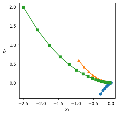
Good news: these validation trajectories can have arbitrarily different length

Xval = [Xval1, Xval2, Xval3]

plt.figure(figsize=(4,4))
plt.plot(Xval1[:,0],Xval1[:,1],'o-')
plt.plot(Xval2[:,0],Xval2[:,1],'^-')
plt.plot(Xval3[:,0],Xval3[:,1],'s-')
plt.xlabel(r'$x_1$')
plt.ylabel(r'$x_2$')

Text(0, 0.5, '$x_2$')

# assemble the trajectories data into a dictionary
validate_data_traj = [{'t':np.arange(tmp.shape[0]), 'x':tmp} for tmp in Xval]

Now, let’s import our modes selection algorithm

from pykoopman.analytics import ModesSelectionPAD21

# feed our model, assembled data dict, and truncation threshold
analysis = ModesSelectionPAD21(model, validate_data_traj, truncation_threshold=1e-3, plot=True)

+-------+--------------------------+------------------------+------------------------+
| Index |        Eigenvalue        |           Q            |           R            |
+-------+--------------------------+------------------------+------------------------+
|   6   | (0.3430000000000002+0j)  | 2.0348468601727288e-14 |   0.5927787679220963   |
|   5   |  (0.699999999999999+0j)  | 1.183399907725707e-13  |  0.12437196865123468   |
|   2   | (0.5600000000000012+0j)  | 1.9861554523348586e-14 |  0.05334173545381721   |
|   0   | (1.0000000000000009+0j)  | 2.094252168112938e-14  |  0.02972174696303384   |
|   3   | (0.48999999999999977+0j) | 2.626657878737818e-14  |  0.01276284982813933   |
|   4   |  (0.799999999999997+0j)  | 1.2125187573675874e-14 | 1.0390418230998807e-15 |
|   8   | (0.4479999999999998+0j)  | 1.0779567706344939e-14 | 1.1514078032288685e-15 |
|   7   |        (0.392+0j)        | 2.8990611938960905e-14 |  8.58500892936008e-15  |
|   1   | (0.6400000000000008+0j)  | 2.7709699327154725e-14 | 2.7465177058838346e-15 |
|   9   | (0.5120000000000001+0j)  | 1.7038660672921586e-13 | 7.455664344886189e-15  |
+-------+--------------------------+------------------------+------------------------+

Conclusion: 1) if I start to sparsify the modes after number 6, it will not improve the performance (of reconstruction) 2) I observed that \(\lambda=0.7\) is contained in the first because it has the lowest linear evolving error 3) And \(\lambda=0.8\) is included at number 6! this is why the reconstruction error drops quickly after 6. 4) almost every eigenvalue here is excellent. simply because the linear evolving error is around machine precision

Therefore, I am going to set \(L=6\), and perform a sweeping of \(\alpha\) to have a family of sparse selected solution

analysis.sweep_among_best_L_modes(L=6, ALPHA_RANGE=np.logspace(-7,1,10), save_figure=False)

+-------+------------------------+------------+------------------------+
| Index |         Alpha          | # Non-zero |  Reconstruction Error  |
+-------+------------------------+------------+------------------------+
|   0   |         1e-07          |     0      |          1.0           |
|   1   | 7.742636826811278e-07  |     1      |  0.49422523882244396   |
|   2   | 5.994842503189409e-06  |     3      |  0.10116573729866045   |
|   3   | 4.641588833612772e-05  |     3      |  0.10116573729866045   |
|   4   | 0.00035938136638046257 |     5      | 1.4444276728552715e-15 |
|   5   | 0.0027825594022071257  |     4      | 1.0362612697620602e-15 |
|   6   |  0.021544346900318822  |     2      | 5.628673469786712e-15  |
|   7   |  0.16681005372000557   |     2      | 5.628673469786712e-15  |
|   8   |   1.2915496650148828   |     2      | 5.628673469786712e-15  |
|   9   |          10.0          |     2      | 5.628673469786712e-15  |
+-------+------------------------+------------+------------------------+

The above plot tells me 1) I just need 2 Koopman modes, I can reconstruct my validation data very well 2) I should select \(\alpha \approx -5\), which corresponds to the index = 6 3) That is to say, the latent dimension is very likely to be 2. Of course.. we know it is a 2D linear system

Let’s get a pruned model

# you need to decide which alpha to choose, from the table above.
# and you need to feed training data (well, you could include validation
# but here I choose to only use training data) into to the command...
pruned_model = analysis.prune_model(i_alpha=6, x_train=X.T)

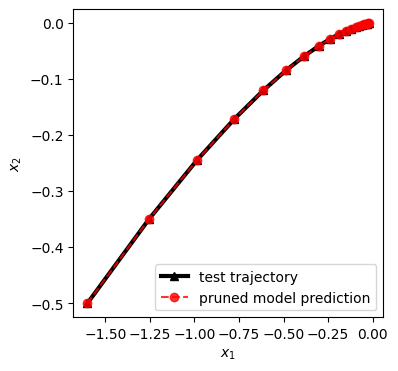
Test the performance of such reduced model on an unseen trajectory

# prepare testing data
n_int_val = 20
n_traj_val = 1
xval = np.array([[-1.6], [-0.5]])
xval_list = []
for i in range(n_int_val):
    xval_list.append(xval)
    xval = sys.linear_map(xval)
Xval4 = np.hstack(xval_list).T

# run simulation on the testing data
x_ = Xval4[0:1,:]
Xval4_pred = []
for i in range(Xval4.shape[0]):
    Xval4_pred.append(x_)
    x_ = pruned_model.predict(x_)
Xval4_pred = np.vstack(Xval4_pred)


plt.figure(figsize=(4,4))
plt.plot(Xval4[:,0],Xval4[:,1],'k^-',alpha=1,label='test trajectory',lw=3)
plt.plot(Xval4_pred[:,0],Xval4_pred[:,1],'ro--',alpha=0.8,label='pruned model prediction')
plt.xlabel(r'$x_1$')
plt.ylabel(r'$x_2$')
plt.legend(loc='best')

<matplotlib.legend.Legend at 0x18481104be0>

Check pruned system methods and matrix

# the number of Koopman modes should be only 2 modes

pruned_model.W.shape

(2, 2)

# compute the eigenfunction along validation trajectory Xval4, there are 2 modes after truncation with 20 snapshots

pruned_model.psi(x_col=Xval4.T).shape

(2, 20)

pruned_model.lamda

array([[0.7+0.j, 0. +0.j],
       [0. +0.j, 0.8+0.j]])