Extended DMD with control for chaotic duffing oscillator

Forced duffing oscillator: This is example adapted from Nathan Kutz’s course https://faculty.washington.edu/kutz/am568/am568.html), with dynamics given by:

\[\begin{split}\dot{x}_{1} = x_2,\\ \dot{x}_2 = -\delta x_2 - \alpha x_1 -\beta x_1^3 + u\end{split}\]

with damped case \(d=0.02,\alpha=-1, \beta=1\)

import sys
sys.path.append('../src')

%matplotlib inline
import pykoopman as pk
from pykoopman.common.examples import forced_duffing, rk4, sine_wave  # required for example system
import matplotlib.pyplot as plt
import numpy as np
import numpy.random as rnd
np.random.seed(42)  # for reproducibility

import warnings
warnings.filterwarnings('ignore')

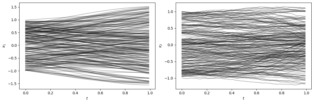
Training data: a training dataset is created consisting of 200 trajectories, each trajectory is integrated for 1000 timesteps and forced by a random actuation in the range \([-1,1]\). Each trajectory starts at a random initial condition in the unit box \([-1,1]^2\).

n_states = 2 # Number of states
n_inputs = 1 # Number of control inputs
dT = 0.01    # Timestep
n_traj = 200  # Number of trajectories
n_int = 1000  # Integration length

d = 0.02   # chaotic case

# Time vector
t = np.arange(0, n_int*dT, dT)

# Uniform random distributed forcing in [-1, 1]
u = 2*rnd.random([n_int, n_traj])-1

# Uniform distribution of initial conditions
x = 2*rnd.random([n_states, n_traj])-1

# Init
U = np.zeros((n_inputs, n_int*n_traj))
U = u.reshape(1,-1)
# Integrate to get data
model_fd = forced_duffing(dt=t[1]-t[0], d=d, alpha=-1, beta=1)
X,Y = model_fd.collect_data_discrete(x, n_int, u)

# Visualize first 100 steps of the training data
fig, axs = plt.subplots(1, 2, tight_layout=True, figsize=(12, 4))
for traj_idx in range(n_traj):
    x = X[:, traj_idx::n_traj]
    axs[0].plot(t[0:100], x[0, 0:100], 'k',alpha=0.3)
    axs[1].plot(t[0:100], x[1, 0:100], 'k',alpha=0.3)
axs[0].set(ylabel=r'$x_1$', xlabel=r'$t$')
axs[1].set(ylabel=r'$x_2$', xlabel=r'$t$')

[Text(0, 0.5, '$x_2$'), Text(0.5, 0, '$t$')]

EDMDc model: The observables (or lifting functions) for the Koopman model are chosen to be the state itself (\(\psi_1 = x_1,\psi_2=x_2\)) (by setting include_states=True below, which is also the default) and thin plate radial basis functions with centers selected randomly.

EDMDc = pk.regression.EDMDc()

centers = np.random.uniform(-1.5,1.5,(2,4))
RBF = pk.observables.RadialBasisFunction(
    rbf_type="thinplate",
    n_centers=centers.shape[1],
    centers=centers,
    kernel_width=1,
    polyharmonic_coeff=1.0,
    include_state=True,
)

model = pk.Koopman(observables=RBF, regressor=EDMDc)
model.fit(X.T, y=Y.T, u=U.T)

Koopman(observables=RadialBasisFunction(centers=array([[-0.95376625,  0.11500887, -1.3650419 , -0.60594909],
       [-1.17360593,  0.36518006,  1.3439246 , -1.36668175]]),
                                        kernel_width=1, n_centers=4,
                                        rbf_type='thinplate'),
        regressor=EDMDc())

In a Jupyter environment, please rerun this cell to show the HTML representation or trust the notebook.
On GitHub, the HTML representation is unable to render, please try loading this page with nbviewer.org.

Compare prediction accuracy of Koopman model on a test trajectory

In the following, the trained model is used to perform a multi-step prediction from a given initial condition. The prediction is compared with the true trajectory when integrating the nonlinear system. Moreover, we will use a sine wave as input signal, which mimics the classic chaotic forced duffing oscillator (where cos wave is used.)

n_int = 3000  # Integration length
t = np.arange(0, n_int*dT, dT)
u = np.array([-sine_wave(step+1) for step in range(n_int)])
x = np.array([0.5, -0.5])
# x = np.array([[-0.1], [-0.5]])

# Integrate nonlinear system


Xtrue = np.zeros((n_states, n_int))
Xtrue[:, 0] = x
Xtrue = model_fd.simulate(Xtrue[:,0:1], n_int, u[:,np.newaxis])

Predict using Koopman model

# Multi-step prediction with Koopman/EDMDc model
Xkoop = model.simulate(x, u[:, np.newaxis], n_steps=n_int-1)
Xkoop = np.vstack([x[np.newaxis,:], Xkoop]) # add initial condition to simulated data for comparison below

Plot the results

fig, axs = plt.subplots(3, 1, sharex=True, tight_layout=True, figsize=(9, 6))
axs[0].plot(t, u, '-k')
axs[0].set(ylabel=r'$u$')
axs[1].plot(t, Xtrue[0, :], '-', color='b', label='True')
axs[1].plot(t, Xkoop[:, 0], '--r', label='EDMDc')
axs[1].set(ylabel=r'$x_1$')
axs[2].plot(t, Xtrue[1, :], '-', color='b', label='True')
axs[2].plot(t, Xkoop[:, 1], '--r', label='EDMDc')
axs[2].set(
        ylabel=r'$x_2$',
        xlabel=r'$t$')
axs[1].legend(loc='best')
axs[1].set_ylim([-2.5,2.5])
axs[2].set_ylim([-2.5,2.5])

(-2.5, 2.5)

Conclusion: 1) the Koopman model is only short time accurate, which makes sense. 2) the Koopman model exhibits simple periodic predictions in the long run

model.A.shape

(6, 6)

model.B.shape

(6, 1)

model.C.shape

(2, 6)

model.W.shape

(2, 6)