Dynamic mode decomposition on two mixed spatial signals

We apply dynamic mode decomposition (DMD) to a spatiotemporal, linear system, which is created as a superposition from two mixed spatiotemporal signals (this is example 1.4 in Kutz et al., “Dynamic Mode Decomposition”, SIAM 2016):

\[f(x,t) = f_1(x,t) + f_2(x,t)\]

with

\[\begin{split}\begin{aligned} f_1(x,t) &= \mathrm{sech}(x+3) e^{j2.3t},\\ f_2(x,t) &= 2\,\mathrm{sech}(x)\,\mathrm{tanh}(x) e^{j2.8t}. \end{aligned}\end{split}\]

These two individual signals have frequencies \(\omega_1 = 2.3\) and \(\omega_2=2.8\) with each a distinct spatial structure.

We first import the pyKoopman package and other packages for plotting and matrix manipulation.

import sys
sys.path.append('../src')

%matplotlib inline
import matplotlib.pyplot as plt
import numpy as np
import warnings
warnings.filterwarnings('ignore')

import matplotlib.cm as cm
from mpl_toolkits.mplot3d import Axes3D

import pykoopman as pk

Time and space discretizations

tArray = np.linspace(0, 4*np.pi, 200)  # Time array for solution
dt = tArray[1] - tArray[0] # Time step
xArray = np.linspace(-10,10,400)
[Xgrid, Tgrid] = np.meshgrid(xArray, tArray)

Define helper function, hyperbolic secant

def sech(x):
    return 1./np.cosh(x)

Generate training data from two spatiotemporal signals

omega1 = 2.3
omega2 = 2.8
f1 = np.multiply(sech(Xgrid+3), np.exp(1j*omega1*Tgrid))
f2 = np.multiply( np.multiply(sech(Xgrid), np.tanh(Xgrid)), 2*np.exp(1j*omega2*Tgrid))
f = f1 + f2

def plot_dynamics(Xgrid, Tgrid, f, fig=None, title='', subplot=111):
    if fig is None:
        fig = plt.figure(figsize=(12, 4))

    time_ticks = np.array([0, 1*np.pi, 2*np.pi, 3*np.pi, 4*np.pi])
    time_labels = ('0', r'$\pi$', r'$2\pi$', r'$3\pi$', r'$4\pi$')

    ax = fig.add_subplot(subplot, projection='3d')
    surf = ax.plot_surface(Xgrid, Tgrid, f, rstride=1)
    cset = ax.contourf(Xgrid, Tgrid, f, zdir='z', offset=-1.5, cmap=cm.ocean)
    ax.set(
        xlabel=r'$x$',
        ylabel=r'$t$',
        title=title,
        yticks=time_ticks,
        yticklabels=time_labels,
        xlim=(-10, 10),
        zlim=(-1.5, 1),
    )
    ax.autoscale(enable=True, axis='y', tight=True)

fig = plt.figure(figsize=(12,4))
fig.suptitle('Spatiotemporal dynamics of mixed signal')

plot_dynamics(Xgrid, Tgrid, f, fig=fig, title=r'$f(x, t) = f_1(x,t) + f_2(x,t)$', subplot=131)
plot_dynamics(Xgrid, Tgrid, f1, fig=fig, title=r'$f_1(x,t)$', subplot=132)
plot_dynamics(Xgrid, Tgrid, f2, fig=fig, title=r'$f_2(x,t)$', subplot=133)

Instantiate and fit a Koopman model using DMD on training data

from pydmd import DMD

dmd=DMD(svd_rank=2)

model = pk.Koopman(regressor=dmd)
model.fit(f, dt=dt)

Koopman(observables=Identity(),
        regressor=PyDMDRegressor(regressor=<pydmd.dmd.DMD object at 0x000001AA579B33A0>))

In a Jupyter environment, please rerun this cell to show the HTML representation or trust the notebook.
On GitHub, the HTML representation is unable to render, please try loading this page with nbviewer.org.

K = model.A

# Let's have a look at the eigenvalues of the Koopman matrix
evals, evecs = np.linalg.eig(K)
evals_cont = np.log(evals)/dt

fig = plt.figure(figsize=(4,4))
ax = fig.add_subplot(111)
ax.plot([0,0], [omega1,omega2],'rs', label='true',markersize=10)
ax.plot(evals_cont.real, evals_cont.imag, 'bo', label='estimated',markersize=5)


ax.set_xlim([-1,1])
ax.set_ylim([2,3])
plt.legend()
plt.xlabel(r'$Re(\lambda)$')
plt.ylabel(r'$Im(\lambda)$')
# print(omega1,omega2)

Text(0, 0.5, '$Im(\\lambda)$')

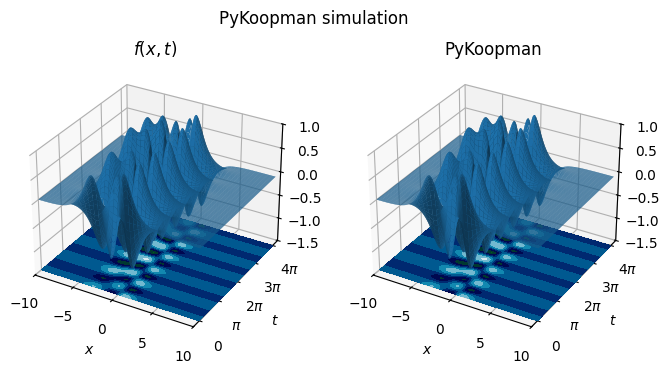
Check if model can reconstruct the training data by predicting starting from the first snapshot.

f_predicted = np.vstack((f[0], model.simulate(f[0], n_steps=f.shape[0] - 1)))

fig = plt.figure(figsize=(8, 4))
fig.suptitle('PyKoopman simulation')

plot_dynamics(Xgrid, Tgrid, f, fig=fig, title=r'$f(x, t)$', subplot=121)
plot_dynamics(Xgrid, Tgrid, f_predicted, fig=fig, title='PyKoopman', subplot=122)