Learning Koopman eigenfunctions on Slow manifold

The linearity, and thus the model performance, of a Koopman model can be analyzed by comparing the linearity of the eigenfunctions evaluated on a test trajectory and the prediction using the corresponding eigenvalue. This will be demonstrated in this tutorial for a two-dimensional system evolving on a slow manifold.

For detailed information we refer to

[1] Kaiser, Kutz & Brunton, “Data-driven discovery of Koopman eigenfunctions for control”, Machine Learning: Science and Technology, Vol. 2(3), 035023, 2021, [2] Korda & Mezic, “Optimal construction of Koopman eigenfunctions for prediction and control”, IEEE Transactions on Automatic Control, Vol. 65(12), 2020.

import sys
sys.path.append('../src')

import pykoopman as pk
import numpy as np
import numpy.random as rnd
np.random.seed(42)  # for reproducibility
import matplotlib.pyplot as plt

np.random.seed(1234)

import warnings
warnings.filterwarnings('ignore')

from pykoopman.common import slow_manifold
nonlinear_sys = slow_manifold(mu=-0.1, la=-1.0, dt=0.1)

Collect training data

n_int = 1
n_pts = 16
xmin = ymin = -2
xmax = ymax = +2
xx, yy = np.meshgrid(np.linspace(xmin, xmax, n_pts), np.linspace(ymin, ymax, n_pts))
Xdat = np.vstack((xx.flatten(), yy.flatten()))

max_n_int = 20

traj_list = []
for i in range(Xdat.shape[1]):
    X, Y = nonlinear_sys.collect_data_discrete(Xdat[:,[i]],
                                               np.random.randint(1, max_n_int))
    tmp = np.hstack([X, Y[:,-1:]]).T
    traj_list.append(tmp)

plt.figure(figsize=(12,4))
plt.bar(np.arange(len(traj_list)), [len(x) for x in traj_list])
plt.xlabel('index of trajectory')
plt.ylabel('number of points in each sequence')
plt.title('we can handle trajectory data with varying-length sequence!')

Text(0.5, 1.0, 'we can handle trajectory data with varying-length sequence!')

test trajectory

x0 = np.array([2, -4])  #np.array([2, -4])
T = 20
t = np.arange(0, T, nonlinear_sys.dt)
Xtest = nonlinear_sys.simulate(x0[:, np.newaxis], len(t)-1).T
Xtest = np.vstack([x0[np.newaxis, :], Xtest])
fig, axs = plt.subplots(2, 1, sharex=True, tight_layout=True, figsize=(12, 6))
axs[0].plot(t, Xtest[:, 0], '-', color='blue', label='True')
axs[0].set(ylabel=r'$x_1$')
axs[1].plot(t, Xtest[:, 1], '-', color='blue', label='True')
axs[1].set(ylabel=r'$x_2$', xlabel=r'$t$')
axs[1].legend(loc='best')

<matplotlib.legend.Legend at 0x1cb819728f0>

plt.figure(figsize=(5,5))

for X in traj_list:
    # for i in range(X.shape[-1]):
    # plt.plot([X[0,i], Y[0,i]], [X[1,i], Y[1,i]],'-k',lw=0.7,label=None)
    plt.plot(X[:,0], X[:,1],'-k', lw=0.7, label=None,alpha=0.1)

# plot test trajectory
plt.plot(Xtest[:, 0], Xtest[:, 1],'-r',label='test')
plt.xlabel(r"$x_1$")
plt.ylabel(r"$x_2$")
plt.title(f"number of training data = {X.shape[-1]} ")
plt.legend(loc='best')

<matplotlib.legend.Legend at 0x1cb819bfac0>

Try EDMD with polynomial features on training data

X_edmd = []
Y_edmd = []
for i in range(len(traj_list)):
    X_edmd.append(traj_list[i][:-1])
    Y_edmd.append(traj_list[i][1:])

X_edmd = np.vstack(X_edmd)
Y_edmd = np.vstack(Y_edmd)

regr = pk.regression.EDMD()
obsv = pk.observables.Polynomial(degree=3)
model_edmd = pk.Koopman(observables=obsv, regressor=regr)
model_edmd.fit(X_edmd, y=Y_edmd, dt=nonlinear_sys.dt)

Koopman(observables=Polynomial(degree=3), regressor=EDMD())

In a Jupyter environment, please rerun this cell to show the HTML representation or trust the notebook.
On GitHub, the HTML representation is unable to render, please try loading this page with nbviewer.org.

koop_eigenvals = np.log(np.linalg.eig(model_edmd.A)[0])/nonlinear_sys.dt

print(f"koopman eigenvalues = {koop_eigenvals}")

koopman eigenvalues = [-1.88130165e+00+0.67548263j -1.88130165e+00-0.67548263j
 -1.65811154e+00+0.j         -3.77475828e-14+0.j
 -9.99991625e-02+0.j         -1.99998325e-01+0.j
 -2.99997487e-01+0.j         -1.09912337e+00+0.j
 -9.99124206e-01+0.j         -6.82569546e-01+0.j        ]

Try NNDMD on training data

look_forward = 20
dlk_regressor = pk.regression.NNDMD(dt=nonlinear_sys.dt, look_forward=look_forward,
                                    config_encoder=dict(input_size=2,
                                                        hidden_sizes=[32] * 3,
                                                        output_size=3,
                                                        activations="swish"),
                                    config_decoder=dict(input_size=3, hidden_sizes=[],
                                                        output_size=2, activations="linear"),
                                    batch_size=1000, lbfgs=True,
                                    normalize=True, normalize_mode='equal',
                                    normalize_std_factor=1.0,
                                    trainer_kwargs=dict(max_epochs=10))

# train the vanilla NN model
model = pk.Koopman(regressor=dlk_regressor)
model.fit(traj_list, dt=nonlinear_sys.dt)

INFO: GPU available: True (cuda), used: True
[rank_zero.py:64 -                _info() ] GPU available: True (cuda), used: True
INFO: TPU available: False, using: 0 TPU cores
[rank_zero.py:64 -                _info() ] TPU available: False, using: 0 TPU cores
INFO: IPU available: False, using: 0 IPUs
[rank_zero.py:64 -                _info() ] IPU available: False, using: 0 IPUs
INFO: HPU available: False, using: 0 HPUs
[rank_zero.py:64 -                _info() ] HPU available: False, using: 0 HPUs
D:\work\pykoopman\venv\lib\site-packages\lightning\pytorch\trainer\configuration_validator.py:69: UserWarning: You passed in a `val_dataloader` but have no `validation_step`. Skipping val loop.
  rank_zero_warn("You passed in a `val_dataloader` but have no `validation_step`. Skipping val loop.")
D:\work\pykoopman\src\pykoopman\regression\_nndmd.py:898: UserWarning: Warning: no validation data prepared
  warn("Warning: no validation data prepared")
INFO: LOCAL_RANK: 0 - CUDA_VISIBLE_DEVICES: [0]
[cuda.py:58 -     set_nvidia_flags() ] LOCAL_RANK: 0 - CUDA_VISIBLE_DEVICES: [0]
INFO:
  | Name                | Type                    | Params
----------------------------------------------------------------
0 | _encoder            | FFNN                    | 2.3 K
1 | _decoder            | FFNN                    | 6
2 | _koopman_propagator | StandardKoopmanOperator | 9
3 | masked_loss_metric  | MaskedMSELoss           | 0
----------------------------------------------------------------
2.3 K     Trainable params
0         Non-trainable params
2.3 K     Total params
0.009     Total estimated model params size (MB)
[model_summary.py:83 -            summarize() ]
  | Name                | Type                    | Params
----------------------------------------------------------------
0 | _encoder            | FFNN                    | 2.3 K
1 | _decoder            | FFNN                    | 6
2 | _koopman_propagator | StandardKoopmanOperator | 9
3 | masked_loss_metric  | MaskedMSELoss           | 0
----------------------------------------------------------------
2.3 K     Trainable params
0         Non-trainable params
2.3 K     Total params
0.009     Total estimated model params size (MB)
D:\work\pykoopman\venv\lib\site-packages\lightning\pytorch\trainer\connectors\data_connector.py:442: PossibleUserWarning: The dataloader, train_dataloader, does not have many workers which may be a bottleneck. Consider increasing the value of the `num_workers` argument` (try 20 which is the number of cpus on this machine) in the `DataLoader` init to improve performance.
  rank_zero_warn(
D:\work\pykoopman\venv\lib\site-packages\lightning\pytorch\loops\fit_loop.py:281: PossibleUserWarning: The number of training batches (1) is smaller than the logging interval Trainer(log_every_n_steps=50). Set a lower value for log_every_n_steps if you want to see logs for the training epoch.
  rank_zero_warn(

INFO: `Trainer.fit` stopped: `max_epochs=10` reached.
[rank_zero.py:64 -                _info() ] `Trainer.fit` stopped: `max_epochs=10` reached.

Koopman(observables=Identity(),
        regressor=NNDMD(batch_size=1000,
                        config_decoder={'activations': 'linear',
                                        'hidden_sizes': [], 'input_size': 3,
                                        'output_size': 2},
                        config_encoder={'activations': 'swish',
                                        'hidden_sizes': [32, 32, 32],
                                        'input_size': 2, 'output_size': 3},
                        dt=0.1, lbfgs=True, look_forward=20,
                        normalize_std_factor=1.0,
                        trainer_kwargs={'max_epochs': 10}))

In a Jupyter environment, please rerun this cell to show the HTML representation or trust the notebook.
On GitHub, the HTML representation is unable to render, please try loading this page with nbviewer.org.

Note: - If you didn’t find the model to converge, that’s because LBFGS is not very robust. You can try again and hope it works again.

Try NNDMD on training data but now we enforce the \(A\) to be disspative

dlk_regressor_d = pk.regression.NNDMD(mode='Dissipative',
                                      dt=nonlinear_sys.dt,
                                      look_forward=look_forward,
                                    config_encoder=dict(input_size=2,
                                                        hidden_sizes=[32] * 3,
                                                        output_size=3,
                                                        activations="swish"),
                                    config_decoder=dict(input_size=3, hidden_sizes=[],
                                                        output_size=2, activations="linear"),
                                    batch_size=1000, lbfgs=True,
                                    normalize=True, normalize_mode='equal',
                                    normalize_std_factor=1.0,
                                    trainer_kwargs=dict(max_epochs=10))

# train the vanilla NN model
model_d = pk.Koopman(regressor=dlk_regressor_d)
model_d.fit(traj_list, dt=nonlinear_sys.dt)

INFO: GPU available: True (cuda), used: True
[rank_zero.py:64 -                _info() ] GPU available: True (cuda), used: True
INFO: TPU available: False, using: 0 TPU cores
[rank_zero.py:64 -                _info() ] TPU available: False, using: 0 TPU cores
INFO: IPU available: False, using: 0 IPUs
[rank_zero.py:64 -                _info() ] IPU available: False, using: 0 IPUs
INFO: HPU available: False, using: 0 HPUs
[rank_zero.py:64 -                _info() ] HPU available: False, using: 0 HPUs
D:\work\pykoopman\venv\lib\site-packages\lightning\pytorch\trainer\configuration_validator.py:69: UserWarning: You passed in a `val_dataloader` but have no `validation_step`. Skipping val loop.
  rank_zero_warn("You passed in a `val_dataloader` but have no `validation_step`. Skipping val loop.")
D:\work\pykoopman\src\pykoopman\regression\_nndmd.py:898: UserWarning: Warning: no validation data prepared
  warn("Warning: no validation data prepared")
INFO: LOCAL_RANK: 0 - CUDA_VISIBLE_DEVICES: [0]
[cuda.py:58 -     set_nvidia_flags() ] LOCAL_RANK: 0 - CUDA_VISIBLE_DEVICES: [0]
INFO:
  | Name                | Type                       | Params
-------------------------------------------------------------------
0 | _encoder            | FFNN                       | 2.3 K
1 | _decoder            | FFNN                       | 6
2 | _koopman_propagator | DissipativeKoopmanOperator | 12
3 | masked_loss_metric  | MaskedMSELoss              | 0
-------------------------------------------------------------------
2.3 K     Trainable params
0         Non-trainable params
2.3 K     Total params
0.009     Total estimated model params size (MB)
[model_summary.py:83 -            summarize() ]
  | Name                | Type                       | Params
-------------------------------------------------------------------
0 | _encoder            | FFNN                       | 2.3 K
1 | _decoder            | FFNN                       | 6
2 | _koopman_propagator | DissipativeKoopmanOperator | 12
3 | masked_loss_metric  | MaskedMSELoss              | 0
-------------------------------------------------------------------
2.3 K     Trainable params
0         Non-trainable params
2.3 K     Total params
0.009     Total estimated model params size (MB)
D:\work\pykoopman\venv\lib\site-packages\lightning\pytorch\trainer\connectors\data_connector.py:442: PossibleUserWarning: The dataloader, train_dataloader, does not have many workers which may be a bottleneck. Consider increasing the value of the `num_workers` argument` (try 20 which is the number of cpus on this machine) in the `DataLoader` init to improve performance.
  rank_zero_warn(
D:\work\pykoopman\venv\lib\site-packages\lightning\pytorch\loops\fit_loop.py:281: PossibleUserWarning: The number of training batches (1) is smaller than the logging interval Trainer(log_every_n_steps=50). Set a lower value for log_every_n_steps if you want to see logs for the training epoch.
  rank_zero_warn(

INFO: `Trainer.fit` stopped: `max_epochs=10` reached.
[rank_zero.py:64 -                _info() ] `Trainer.fit` stopped: `max_epochs=10` reached.

Koopman(observables=Identity(),
        regressor=NNDMD(batch_size=1000,
                        config_decoder={'activations': 'linear',
                                        'hidden_sizes': [], 'input_size': 3,
                                        'output_size': 2},
                        config_encoder={'activations': 'swish',
                                        'hidden_sizes': [32, 32, 32],
                                        'input_size': 2, 'output_size': 3},
                        dt=0.1, lbfgs=True, look_forward=20, mode='Dissipative',
                        normalize_std_factor=1.0,
                        trainer_kwargs={'max_epochs': 10}))

In a Jupyter environment, please rerun this cell to show the HTML representation or trust the notebook.
On GitHub, the HTML representation is unable to render, please try loading this page with nbviewer.org.

Check the continuous eigenvalues

The eigenvalues identified is pretty close… to the ground truth. Although the dissipative one is less accurate, it guarantees stability, which can be very important for uncertainty quantification, and long time stability predictions.

koop_eigenvals = np.log(np.linalg.eig(model.A)[0])/nonlinear_sys.dt
print(f"koopman eigenvalues = {koop_eigenvals}")

koop_eigenvals = np.log(np.linalg.eig(model_d.A)[0])/nonlinear_sys.dt
print(f"koopman eigenvalues with dissipative enforcement = {koop_eigenvals}")

koopman eigenvalues = [-0.99603385 -0.10004931 -0.20210291]
koopman eigenvalues with dissipative enforcement = [-0.9720626  -0.09937927 -0.21690993]

Evaluate model performance on test trajectory

model_d.ur

array([[ 0.4801627 , -0.06952379, -0.07016307],
       [ 0.0335696 , -2.7245688 ,  0.4008407 ]], dtype=float32)

Xkoop_edmd = model_edmd.simulate(x0, n_steps=len(t)-1)
Xkoop_edmd = np.vstack([x0[np.newaxis,:], Xkoop_edmd])

Xkoop_nn_d = model_d.simulate(x0, n_steps=len(t)-1)
Xkoop_nn_d = np.vstack([x0[np.newaxis,:], Xkoop_nn_d])

Xkoop_nn = model.simulate(x0, n_steps=len(t)-1)
Xkoop_nn = np.vstack([x0[np.newaxis,:], Xkoop_nn])

fig, axs = plt.subplots(2, 1, tight_layout=True, figsize=(6, 6))
axs[0].plot(t, Xtest[:, 0], '-', color='k', label='True')
axs[0].plot(t, Xkoop_edmd[:, 0], '--r', label='EDMD')
axs[0].plot(t, Xkoop_nn[:, 0], '--g', label='NNDMD')
axs[0].plot(t, Xkoop_nn_d[:, 0], '--b', label='NNDMD-dissipative')

axs[0].set(ylabel=r'$x_1$')
axs[1].plot(t, Xtest[:, 1], '-', color='k', label='True')
axs[1].plot(t, Xkoop_edmd[:, 1], '--r', label='EDMD')
axs[1].plot(t, Xkoop_nn[:, 1], '--g', label='NNDMD')
axs[1].plot(t, Xkoop_nn_d[:, 1], '--b', label='NNDMD-dissipative')
axs[1].set(ylabel=r'$x_2$', xlabel=r'$t$')
axs[1].legend(loc='best')

axs[1].set_ylim([-4,4])

(-4.0, 4.0)

Evaluate linearity of identified Koopman eigenfunctions

Koopman eigenfunctions evolve linearly in time and must satisfy:

\[\phi(x(t)) = \phi(x(0)) \exp(\lambda t)\]

It is possible to evaluate this expression on a test trajectory \(x(t)\) with a linearity error defined by:

\[e = \Vert \phi(x(t)) - \phi(x(0)) \exp(\lambda t) \Vert\]

efun_index, linearity_error = model_edmd.validity_check(t, Xtest)
print("Ranking of eigenfunctions by linearity error: ", efun_index)
print("Corresponding linearity error: ", linearity_error)

Ranking of eigenfunctions by linearity error:  [4 7 6 8 3 5 1 0 2 9]
Corresponding linearity error:  [1.787183161285686e-12, 3.60789557348859e-12, 1.0079736747933206e-11, 1.016677184845744e-11, 1.9276821336498066e-11, 2.0840686600530602e-11, 25.40265614296923, 25.402656142969267, 25.594030653971245, 110.7878547958471]

efun_index, linearity_error = model.validity_check(t, Xtest)
print("Ranking of eigenfunctions by linearity error: ", efun_index)
print("Corresponding linearity error: ", linearity_error)

Ranking of eigenfunctions by linearity error:  [1 0 2]
Corresponding linearity error:  [0.08088682341571321, 0.08260710527483629, 0.18168451100968588]

efun_index, linearity_error = model_d.validity_check(t, Xtest)
print("Ranking of eigenfunctions by linearity error: ", efun_index)
print("Corresponding linearity error: ", linearity_error)

Ranking of eigenfunctions by linearity error:  [0 1 2]
Corresponding linearity error:  [0.29899081987665693, 0.38791952389950124, 2.0498793587778]

Observation

You can see NN-DMD with one step optimizatin is not giving you the theoretical result. Although such model seems to fit the trajectory very well.

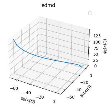
Further, in below, you can see the EDMD eigenfunction can be huge because we are simply using monomials.

Visualization of eigenfunction on test trajectory

from mpl_toolkits.mplot3d import Axes3D

phi_edmd_test = model_edmd.psi(Xtest.T)
phi_nn_test = model.psi(Xtest.T)
phi_nn_d_test = model_d.psi(Xtest.T)

title_list = ['edmd','nndmd','nndmd-dissipative']
phi_list = [phi_edmd_test, phi_nn_test, phi_nn_d_test]

for i in range(3):
    phi = phi_list[i]
    fig = plt.figure(figsize=(4,4))
    ax = fig.add_subplot(111, projection='3d')
    ax.plot(np.real(phi)[0,:],np.real(phi)[1,:],np.real(phi)[2,:])
    ax.set_xlabel(r'$\psi_0(x(t))$')
    ax.set_ylabel(r'$\psi_1(x(t))$')
    ax.set_zlabel(r'$\psi_2(x(t))$')

    plt.title(title_list[i])
    plt.legend(loc='best')

[legend.py:1217 -   _parse_legend_args() ] No artists with labels found to put in legend.  Note that artists whose label start with an underscore are ignored when legend() is called with no argument.
[legend.py:1217 -   _parse_legend_args() ] No artists with labels found to put in legend.  Note that artists whose label start with an underscore are ignored when legend() is called with no argument.
[legend.py:1217 -   _parse_legend_args() ] No artists with labels found to put in legend.  Note that artists whose label start with an underscore are ignored when legend() is called with no argument.

Access the matrices related to Koopman operator

model.A.shape

(3, 3)

model.C.shape

(2, 3)

model.W.shape

(2, 3)